Interest Rate Model (IRM)

Configure utilization-based or fixed rate models

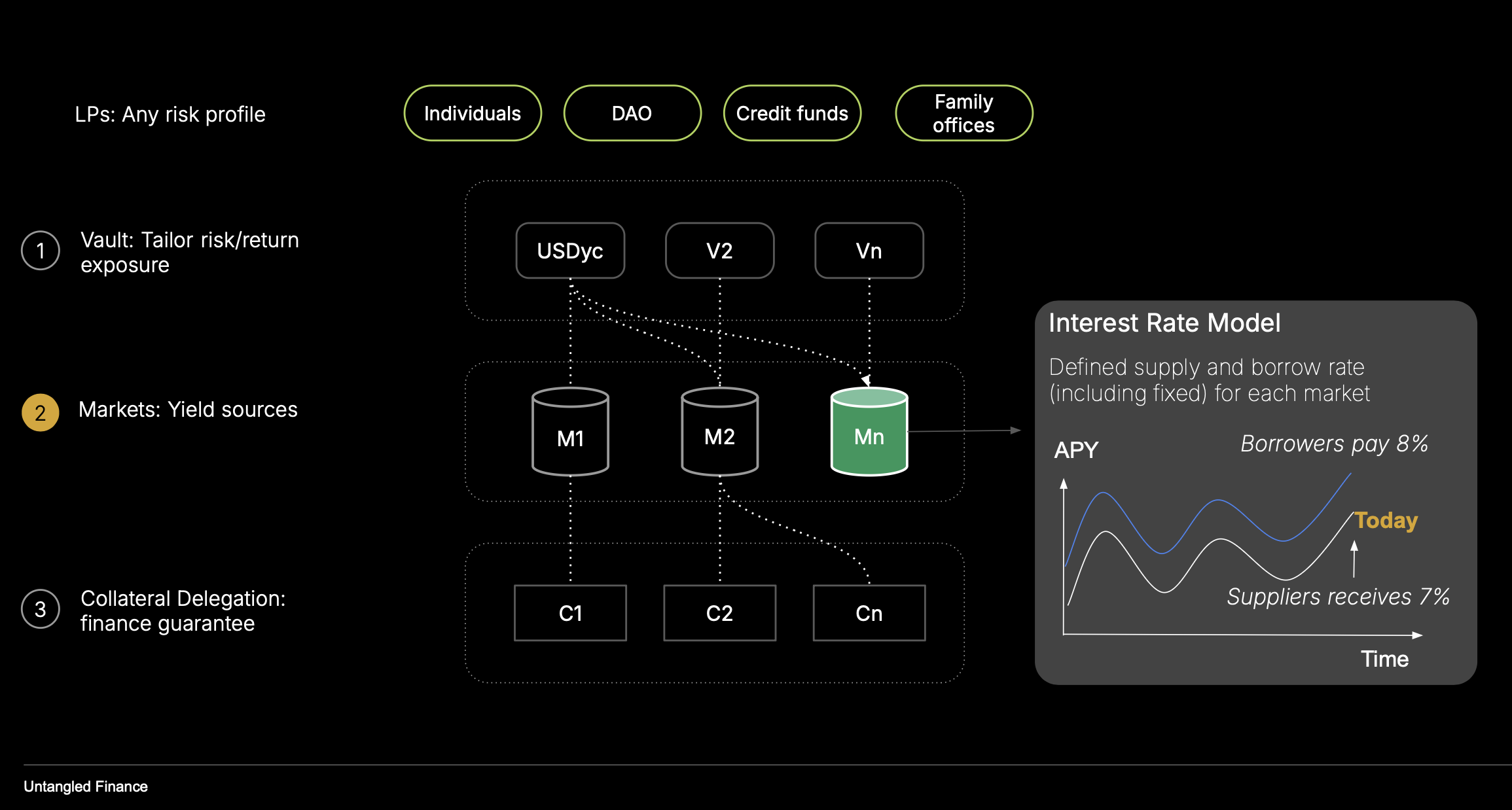
Overview

OctoLend’s Interest Rate Model (IRM) governs how borrowing costs evolve over time, targeting liquidity resilience across market conditions.

The model combines:

• A utilization-linked baseline (linear floor).
• A stabilizing integral term around an optimal utilization.
• An adaptive penalty that accelerates rates above a critical utilization threshold.
• A low-utilization dampener to avoid overpricing when markets are underused.

The IRM produces both an instantaneous annualized rate (for pricing) and a compounded effect over time (for debt growth and debt-share pricing). It anchors rates to a linear utilization floor, stabilizes around an optimal target, and escalates dynamically above a critical threshold with time-decaying memory.

By pairing instantaneous pricing with explicit compounding, the IRM balances liquidity, predictability, and responsiveness—key for institutional-grade lending on OctoLend.

Purpose

The IRM’s goal is to keep markets liquid and predictable:

• Encourage repayments or fresh supply when utilization is high.
• Avoid punitive rates when utilization is low.
• Stabilize around a curator-chosen optimal utilization (at market initialization).
• Adapt quickly during stress while decaying back when conditions normalize.

This aligns vault liquidity with user withdrawals and protects lenders from prolonged max-utilization states.

What the IRM Controls

• Instantaneous borrow rate (annualized): Derived from current utilization and state variables.
• Compounded growth: Total debt assets between accruals.
• Debt price: Value per debt share (debt assets per debt share).
• Internal adaptation variables: Govern how quickly the system responds or cools around critical utilization.

Key Parameters

Each market sets a one-time configuration. Parameters are expressed in fixed-point integers (WAD = 1e18) or integers/basis points as appropriate.

Parameter	Description
u_opt	Target (optimal) utilization. Nudges rates to maintain balance near this level.
u_crit	Critical utilization where penalty component activates.
u_low	Low-utilization floor; applies dampener to prevent overpricing.
k_lin	Baseline slope for linear utilization-linked rate (r_lin = k_lin × u).
k_i	Integral gain toward u_opt; accumulates pressure to return to target.
k_crit	Penalty slope above u_crit; controls aggressiveness of rate escalation.
k_low	Low-utilization slope shaping rate depression below u_low.
beta	Adaptation speed of stress memory (t_crit).
r_i	Internal baseline rate (stateful), updated per accrual.
t_crit	Stateful stress memory term; ramps up above u_crit and decays below.

Parameters and bindings are immutable once the market is initialized.

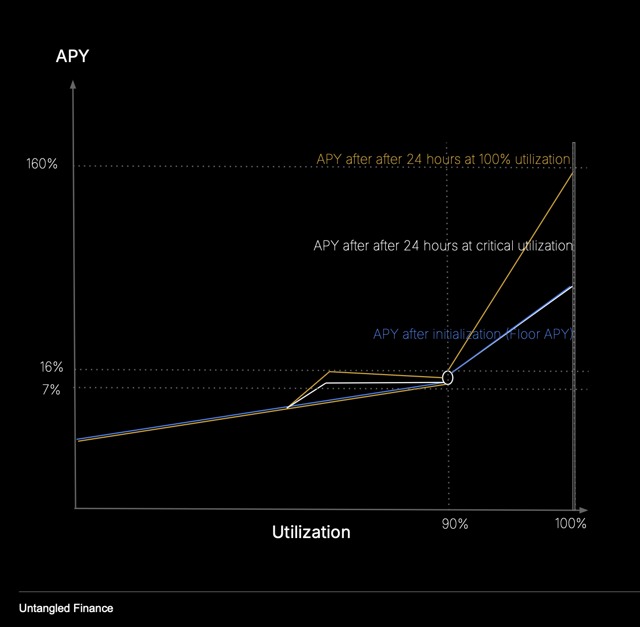
Rate Dynamics

Linear Baseline

r_lin = k_lin × u
Rates grow linearly with utilization, ensuring a utilization-appropriate floor.

Integral Stabilization around u_opt

The internal baseline r_i adjusts over time using (u − u_opt):

• If utilization > u_opt, r_i increases.
• If utilization < u_opt, r_i decreases (bounded by r_lin).
  This slow correction keeps utilization near the target.

Stress Penalty above u_crit

When utilization exceeds u_crit, a penalty r_p activates:

• The longer utilization stays above u_crit, the higher the stress memory (t_crit).
• As t_crit builds, rates increase to attract liquidity or force repayments.
• When utilization normalizes, t_crit decays at a beta-controlled rate.

Low-Utilization Dampener

When utilization drops below u_low, a capped negative adjustment prevents excessive rates in quiet markets.

Putting It Together

The model combines all rate components and takes:
r = max(r_lin, r_i + r_p)
This per-second rate is scaled to an annualized figure for display.

Compounding and Accrual

Between accrual timestamps, the IRM integrates the evolving rate to produce a compounded growth factor for total debt:

1. Approximates rate path between last accrual and now (piecewise-linear).
2. Exponentiates integrated value to obtain compounded factor r_comp (in WAD).
3. Updates total debt assets: total_debt = total_debt × (1 + r_comp).

This captures both gradual stabilization (integral term) and rapid stress responses (penalty term).

Debt Price and Debt Shares

The IRM provides a debt price used to value borrower debts:

• Reflects total debt assets, compounded factor, and total debt shares outstanding.
• If no debt shares exist yet, a fixed initial price is returned.
• The price increases with accrued interest, ensuring accurate valuation for accounting and liquidations.

This gives curators and analysts transparent insight into market health.

Initialization and Lifecycle

• Bound to a specific lending market at deployment.
• Configuration is immutable for predictability.
• On first use, IRM records total debt assets and starts its accrual clock.

Each accrue call:

1. Updates t_crit and r_i.
2. Advances last accrual timestamp.
3. Compounds total debt assets by the new growth factor.

Outputs

• Instantaneous rate (annualized) Current borrowing APR implied by utilization and model state.
• Compounded factor Growth of debt since the last accrual interval.
• Debt price Value per debt share for accounting and liquidation.

These metrics show liquidity pressure and verify the IRM’s responsiveness.

Safety and Guardrails

• Floors and bounds: Rates never fall below r_lin.
• Memory decay: Stress memory (t_crit) cools when utilization normalizes.
• Fixed-point math: Deterministic arithmetic avoids rounding errors.
• Immutable configuration: Prevents mid-lifecycle governance drift.

What to Monitor

• Utilization: Compare u vs. u_opt and u_crit.
• Stress memory (t_crit): Indicates if stress conditions persist.
• Rate behavior: Check r_lin vs. current rate to observe adjustments.
• Accrual cadence: Ensure compounding matches utilization changes.
• Debt price vs. repayments: Validate accounting consistency.

Example Behaviors

Market Condition	Behavior
Quiet (u < u_opt)	Rates hover near r_lin; integral nudges utilization upward.
Efficient (u ≈ u_opt)	Rates stable; minor deviations corrected smoothly.
Stress (u > u_crit)	Penalty activates; rates climb quickly; decays as utilization normalizes.

FAQs

Does the model support fixed rates?
Yes. OctoLend supports fixed-rate configurations via a separate IRM profile, selectable at market creation.

Why not a single kinked curve?
Traditional kinked curves are static. OctoLend’s IRM adds time-dependent memory and an integral term, allowing dynamic stress adaptation and smoother normalization.

How often should accrual run?
Accrual can be called whenever meaningful time or utilization change occurs. Frequent accrual captures rate dynamics more accurately.

What happens at extremely low utilization?
The low-utilization dampener ensures borrowing costs remain attractive, preventing stagnation in underused markets.

Configurations

Dynamic Kink with PI Controller

Defines an optimal utilization band with stable rates. Beyond it, rates move dynamically to restore balance, attracting deposits or encouraging repayments.

Dynamic Kink (Linear)

Rates rise linearly with utilization up to a critical threshold, then increase more sharply.

Fixed

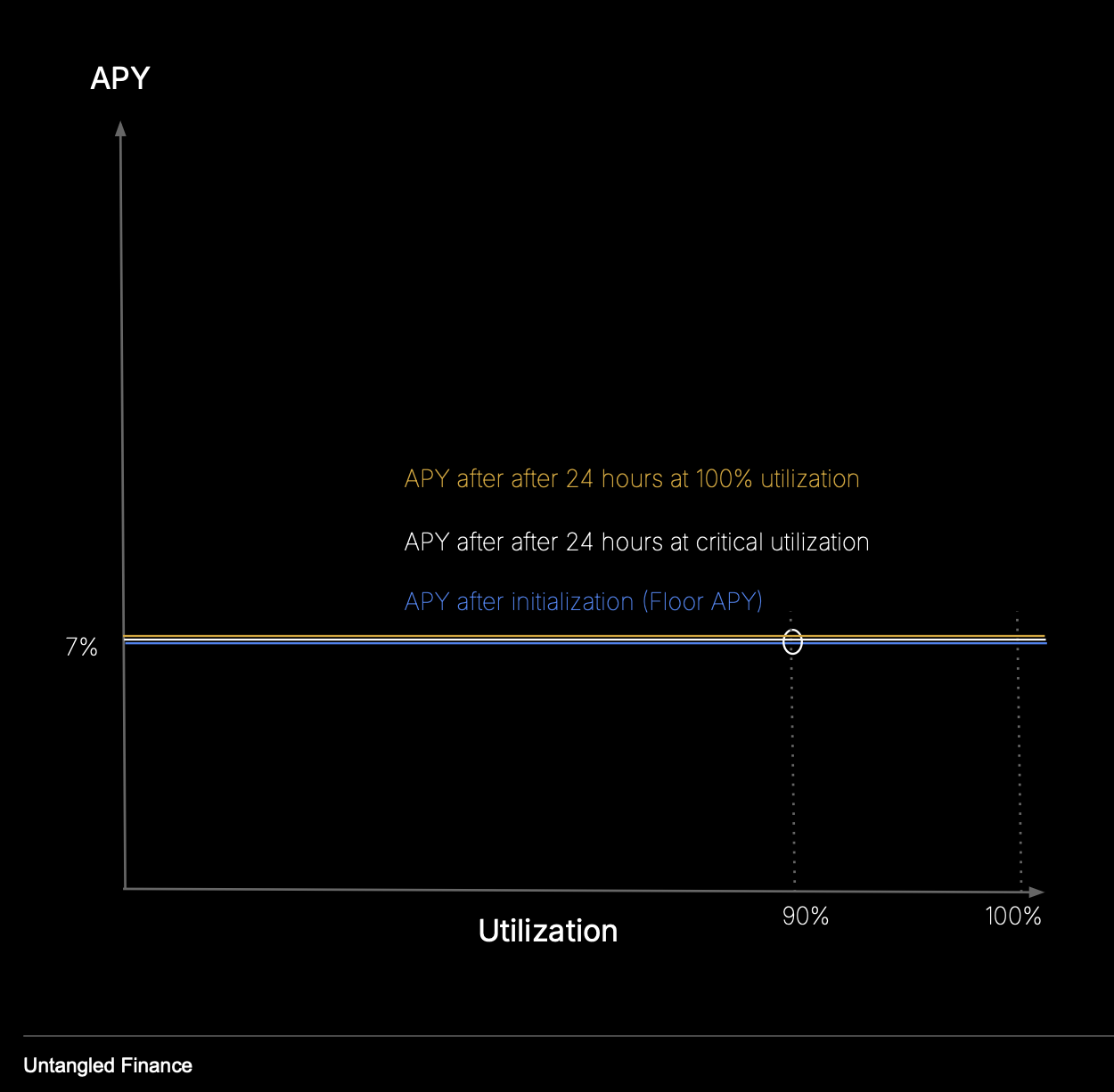
Borrow rate is constant across all utilization levels — ideal for fixed-rate or RWA-style markets.